An experiment to extend the three.js boids example with a dynamic targets. These target positions are determined by solving for the catenary connecting user controlled points while the boid targeting motion involved weighting the boid velocities computed in parallel as a fragment shader.
Catenary between Points
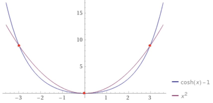
A catenary describes the shape of an idealized chain or cable hanging between two points.
\[ y = a \cosh{ \frac{x}{a} } \]
While similar in shape to a parabola, a catenary that has non-zero intersections with a parabola will have relatively smaller values between these intersection points, giving it a slight bulge in comparison. Although hard to tell apart independently, when overlaid in the above plot, the parabola feels as though it is under tension as if being stretched by the intersection points while the catenary has been allowed to settle under the weight of the chain.
The catenary can be generalized to any offset in \(\mathbb{R}^2\),
\[ y = a \cosh{ \frac{x - b}{a} } + c \]
so that our goal is to solve for \(a\), \(b\), and \(c\) given two points along this curve and the length of wire between them.
Finding a
Let our two points be \((x_1, y_1)\) and \((x_2, y_2)\) such that \(\Delta x = |x_1 - x_2|\) and \(\Delta y = |y_1 - y_2|\). Using the expression relating horizontal and vertical distances between points as well as the curve length \(s\),
\[ \sqrt{s^2 - \Delta y^2} = 2a \sinh{ \frac{ \Delta x }{ 2a } } \]
We would like to solve for \(a\), but it doesn't take much juggling of \(\sinh\) to discover that this transcendental equation in \(a\) doesn't have an analytic solution so we'll approximate \(\sinh\) using the Taylor Series expansion.
\[ \sinh x = x + \frac {x^3} {3!} + \frac {x^5} {5!} + \frac {x^7} {7!} +\cdots = \sum_{n=0}^\infty \frac{x^{2n+1}}{(2n+1)!} \]
Using the first three terms as our approximation,
\[ \sinh{ \frac{ \Delta x }{ 2a } } \approx \frac{ \Delta x }{ 2a } + \frac{1}{3!} \left( \frac{ \Delta x }{ 2a } \right)^3 + \frac{1}{5!} \left( \frac{ \Delta x }{ 2a } \right) ^5 \]
\[ \Rightarrow \sqrt{s^2 - \Delta y^2} \approx 2a \left( \frac{ \Delta x }{ 2a } + \frac{1}{3!} \left( \frac{ \Delta x }{ 2a } \right)^3 + \frac{1}{5!} \left( \frac{ \Delta x }{ 2a } \right) ^5 \right) \]
Rearranging and a bit of simplifying,
\[ 0 \approx \Delta x + \frac{ \Delta x^3 }{ 3!(2a)^2 } + \frac{ \Delta x^5 }{ 5!(2a)^4 } - \sqrt{s^2 - \Delta y^2} \]
\[ 0 \approx \left( \Delta x - \sqrt{s^2 - \Delta y^2} \right) (2a)^4 + \frac{ \Delta x^3 }{ 3! } (2a)^2 + \frac{ \Delta x^5 }{ 5! } \]
And if we let \(u = (2a)^2\),
\[ 0 \approx \left( \Delta x - \sqrt{s^2 - \Delta y^2} \right) u^2 + \frac{ \Delta x^3 }{ 3! } u + \frac{ \Delta x^5 }{ 5! } \]
To solve for \(a\), \(u\) must be positive, so we focus on the positive solution to the quadratic,
\[ u \approx \frac{-b + \sqrt{ b^2 - 4dc }}{2d} \]
where,
\[ \begin{aligned} d &= \Delta x - \sqrt{s^2 - \Delta y^2} \\ b &= \frac{ \Delta x^3 }{ 3! } \\ c &= \frac{ \Delta x^5 }{ 5! } \end{aligned} \]
Using \(a=\frac{\sqrt{u}}{2}\) we finally have our approximate solution,
\[ a \approx \frac{1}{2}\sqrt{\frac{-b + \sqrt{ b^2 - 4dc }}{2d}} \]
Finding b
Using our generalized equation above, we have one equation for each point,
\[ y_n = a \cosh{ \frac{x_n - b}{a}} + c \]
So it follows that by using two points and our previously found value of \(a\),
\[ y_1 - y_2 = a \cosh{ \frac{x_1 - b}{a}} - a \cosh{ \frac{x_2 - b}{a}} \]
Again, trying to solve for \(b\) analytically will result in a minor case of madness, so we turn to Newton's method for a numerical solution to the zero crossing.
\[ \begin{aligned} f(b) &= a \cosh{ \frac{x_1 - b}{a}} - a \cosh{ \frac{x_2 - b}{a}} + y_2 - y_1 \\ f'(b) &= - a \sinh{ \frac{x_1 - b}{a}} + a \sinh{ \frac{x_2 - b}{a}} \end{aligned} \]
And we iterate the recurrence,
\[ x_{n+1} = x_n - \frac{f(x_n)}{f'(x_n)} \]
until \(f(x_n) \approx 0\).
Finding c
Given that we have already found approximate \(a\) and \(b\), we can finally approximate \(c\) using our generalized equation,
\[ y = a \cosh{ \frac{x - b}{a} } + c \]
By rearranging the terms and using any point \((x_n, y_n)\), we finally have,
\[ c = a \cosh{ \frac{x_n - b}{a} } - y_n \]
Summary
Finding an approximation to one term unlocks the approximation of another. Stringing these together allows us to find the approximate catenary with a given length \(s\) that passes through \((x_1, y_1)\) and \((x_2, y_2)\).
function catenary(x1, y1, x2, y2, s) {
  // Return parameters for catenary of form:
  // y = a * cosh((x - b)/a) + c
  let dx = Math.abs(x1 - x2);
  let dy = Math.abs(y1 - y2);

  // find a using the equation relating dx, dy and s
  // sqrt(s^2 - dy^2) = 2*a*sinh(dx/(2*a))
  // via taylor series to expansion of sinh and solve quadratic for u = (2a)^2
  let ua = dx - Math.sqrt(s*s - dy*dy);
  let ub = dx**3/6;
  let uc = dx**5/120;
  let u = (-ub - Math.sqrt(ub*ub - 4*ua*uc))/(2*ua);
  let a = Math.sqrt(u)/2;

  // use newton's method to find b where
  // y1 = a * cosh((x1-b)/a) + c
  // y2 = a * cosh((x2-b)/a) + c
  let fb  = b => a*Math.cosh((x2 - b)/a) - a*Math.cosh((x1 - b)/a) - y2 + y1;
  let fbp = b => -Math.sinh((x2 - b)/a) + Math.sinh((x1 - b)/a);
  let b = newtonRaphson(fb, fbp, (x1 + x2)/2, {maxIterations: 50});

  // solve for c
  // y1 = a * cosh((x1-b)/a) + c
  let c = y1 - a * Math.cosh((x1 - b)/a)

  return [a, b, c];
}
In practice, you'll want to either ensure that the given points aren't more than \(s\) distance apart or update \(s\) to be the larger of that distance or the given curve length.
Boid targeting
The original boid example contains a fragment shader to compute the velocity (direction and magnitude) of each boid on every frame. This is performed for a single boid by iterating through every other boid and computing the distance between the two. Depending on this distance, the velocity of the boid of interest may be weighted for any of the following:
- separation to avoid another boid
- alignment to steer in the same direction of another boid
- cohesion to move towards another boid
The example also contains a constant weighting towards the center of the screen so the boids remain within view as well as separation from a mouse movement "predator".
To simulate boids landing on a wire, individual boid targeting was added to replace the general center weight. These target locations are created by selecting a random wire and choosing a random \(x\) value between the endpoints of that wire. Using the generalized catenary equation we can then find the actual \((x, y)\) point on that wire that becomes the target location. By generating target locations for every boid passed as a uniform array to the boid vector fragment shader, the boids can be directed to targets with weighting controlled by the distance to the target.